Examples
Example #1
In this example we will use Fictitious Play to solve the Beach Bar environment. We will set the verbose parameter to 5 to view a status printout every five iterations.
[1]:
from mfglib.env import Environment
from mfglib.alg import FictitiousPlay

env = Environment.beach_bar()
alg = FictitiousPlay(alpha=0.13)

_ = alg.solve(env, verbose=True, print_every=5)
┏━━━━━━━━━━━━━━━━━━━━━━━━━━━━━━━━━━━━━━━━━━━━━━━━━━━━━━━━━━━┓
┃                                                           ┃
┃      MFGLib v0.3.0 : A Library for Mean-Field Games       ┃
┃              RADAR Research Lab, UC Berkeley              ┃
┃                                                           ┃
┗━━━━━━━━━━━━━━━━━━━━━━━━━━━━━━━━━━━━━━━━━━━━━━━━━━━━━━━━━━━┛
┌─ Environment Summary ─────────────────────────────────────┐
│ S = (4,)                                                  │
│ A = (3,)                                                  │
│ T = 2                                                     │
│ r_max = 4                                                 │
└───────────────────────────────────────────────────────────┘
┌─ Algorithm Summary ───────────────────────────────────────┐
│ class = FictitiousPlay                                    │
│ parameters = {'alpha': 0.13}                              │
│ atol = 0.001                                              │
│ rtol = 0.001                                              │
│ max_iter = 100                                            │
└───────────────────────────────────────────────────────────┘
┌─ Documentation ───────────────────────────────────────────┐
│ - Ratio_n := Expl_n / Expl_0.                             │
│ - Argmin_n := Argmin_{0≤i≤n} Expl_i.                      │
│ - Elapsed_n measures time in seconds.                     │
└───────────────────────────────────────────────────────────┘
┏━━━━━━━━━━┳━━━━━━━━━━━━┳━━━━━━━━━━━━┳━━━━━━━━━━┳━━━━━━━━━━━┓
┃ Iter (n) ┃ Expl_n     ┃ Ratio_n    ┃ Argmin_n ┃ Elapsed_n ┃
┡━━━━━━━━━━╇━━━━━━━━━━━━╇━━━━━━━━━━━━╇━━━━━━━━━━╇━━━━━━━━━━━┩
│ 0        │ 1.2213e+00 │ 1.0000e+00 │ 0        │ 0.00e+00  │
│ 5        │ 3.8416e-01 │ 3.1456e-01 │ 5        │ 9.29e-03  │
│ 10       │ 1.5814e-01 │ 1.2949e-01 │ 10       │ 1.69e-02  │
│ 15       │ 7.3824e-02 │ 6.0449e-02 │ 15       │ 2.43e-02  │
│ 20       │ 3.8312e-02 │ 3.1371e-02 │ 20       │ 3.16e-02  │
│ 25       │ 2.3232e-02 │ 1.9023e-02 │ 24       │ 3.90e-02  │
│ 30       │ 1.4415e-02 │ 1.1803e-02 │ 29       │ 4.67e-02  │
│ 35       │ 1.1469e-02 │ 9.3912e-03 │ 34       │ 5.41e-02  │
│ 40       │ 4.1311e-03 │ 3.3826e-03 │ 40       │ 6.14e-02  │
│ 45       │ 3.3686e-03 │ 2.7583e-03 │ 45       │ 6.93e-02  │
│ 47       │ 1.4827e-03 │ 1.2141e-03 │ 47       │ 7.23e-02  │
└──────────┴────────────┴────────────┴──────────┴───────────┘
Status: Absolute or relative stopping criteria met.
Example #2
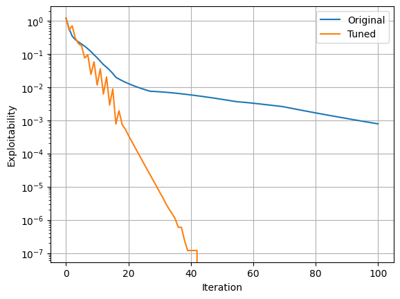
In this example we will demonstrate how to use the tuning API to identify optimal hyperparameters for MF-OMI on the Beach Bar environment. While we will use MF-OMI in this demonstration, it is important to note that all algorithms may benefit from tuning.
[2]:
import matplotlib.pyplot as plt
import optuna

from mfglib.env import Environment
from mfglib.alg import OccupationMeasureInclusion
from mfglib.tuning import GeometricMean

# By default, optuna displays logs. This silences them.
optuna.logging.set_verbosity(optuna.logging.WARNING)

env = Environment.beach_bar()

# initialize algorithm
alg_orig = OccupationMeasureInclusion(alpha=0.09)

# note; atol=rtol=None would turn off early stop and let iterations continue to max_iter
_, expls_orig, _ = alg_orig.solve(env, atol=1e-8, rtol=1e-8)

# tune() returns an optuna.Study object; can use solve_kwargs to match tuner inner solve behavior and final solve behavior
study = alg_orig.tune(metric=GeometricMean(shift=0.5), envs=[env], n_trials=40, solve_kwargs={"atol":1e-8, "rtol": 1e-8})

# which we can use to initialize a new instance
alg_tuned = alg_orig.from_study(study)

_, expls_tuned, _ = alg_tuned.solve(env, atol=1e-8, rtol=1e-8)

plt.xlabel("Iteration")
plt.ylabel("Exploitability")
plt.plot(expls_orig, label="Original")
plt.plot(expls_tuned, label="Tuned")
plt.semilogy()
plt.grid()
plt.legend();
Matplotlib is building the font cache; this may take a moment.
Example #3
In this example we will use Online Mirror Descent to solve the Building Evacuation and visualize how the population behaves under the optimal policy found.
[3]:
import numpy as np

from mfglib.env import Environment
from mfglib.alg import OnlineMirrorDescent
from mfglib.utils import mean_field_from_policy

N_TIMESTEPS = 20
N_FLOORS = 3
SIZE = 8

env = Environment.building_evacuation(
    T=N_TIMESTEPS,
    n_floor=N_FLOORS,
    floor_l=SIZE,
    floor_w=SIZE,
    eta=0.1,
)
alg = OnlineMirrorDescent(alpha=5e-3)

pis, expls, _ = alg.solve(env, atol=None, rtol=None, max_iter=1000)

# Identify the index of the "best" policy, as measured by exploitability
i = np.argmin(expls)

# Compute the corresponding mean-field and state marginal
L_i = mean_field_from_policy(pis[i], env=env)
mu_i = L_i.sum(dim=-1)
For any state \(s = (x, y, z) \in \mathbb{Z}_+^3\) representing a position in the building (\(z\) being the height) let
denote the population state marginal at time \(t\) of the induced mean-field \(L^{\pi^i}\) where \(\pi^i\) is the \(i\)’th policy iterate. Below we plot the population’s state distribution at various times \(t\) as a heatmap.
[4]:
from matplotlib.colors import LogNorm

T_PNTS = [0, N_TIMESTEPS // 2, N_TIMESTEPS]

vmin = mu_i[T_PNTS].min().item()
vmax = mu_i[T_PNTS].max().item()

norm = LogNorm(vmin=vmin + 1e-12, vmax=vmax, clip=True)

fig, axs = plt.subplots(
    nrows=len(T_PNTS), ncols=N_FLOORS, sharex=True, sharey=True, layout="constrained"
)
ims = []
for j, t in enumerate(T_PNTS):
    for z in range(N_FLOORS):
        im = axs[j, z].imshow(mu_i[t, z], norm=norm)
        ims += [im]
        axs[j, z].set_xlabel("x")
        axs[j, z].set_ylabel("y")
        axs[j, z].set_title(rf"$\mu_{{{t}}}^i(x, y, {z})$")

fig.colorbar(ims[0], ax=axs.ravel().tolist())

plt.show()
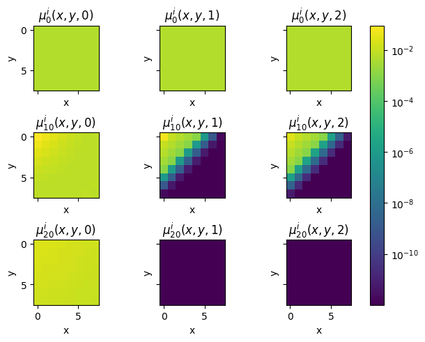
On the top line we see the population evenly distributed throughout the building. In the second line we see the population making their way to the stairs. And the bottom line indicates that the building is fully evacuated at time \(t = 20\).