A Library for Mean-Field Games
Installation
MFGLib provides pre-built wheels for Python 3.8+ and can be installed via pip on
all major platforms:
$ pip install mfglib
Additionally, the source code is directly available on GitHub.
Your First MFG
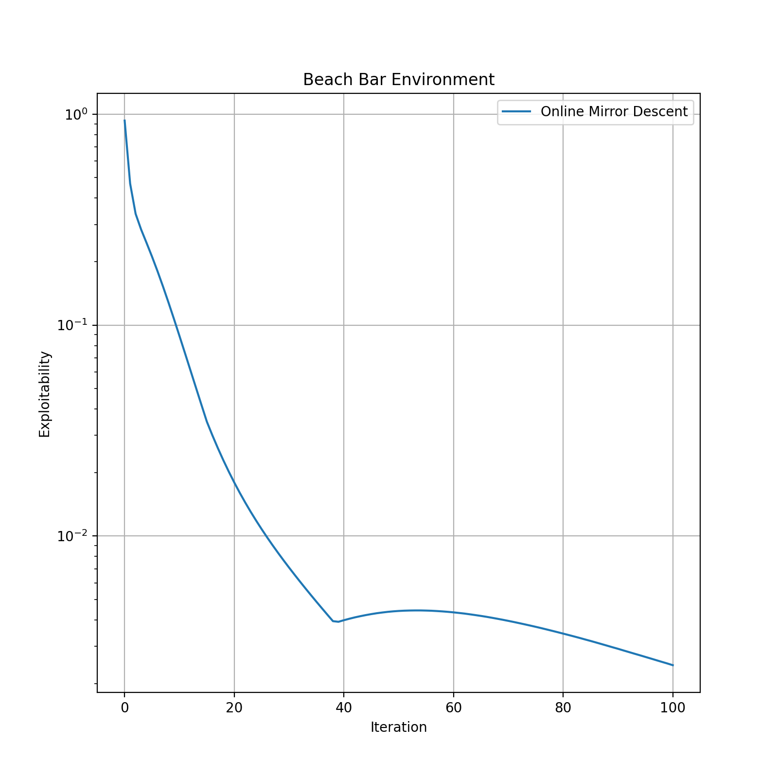
To demonstrate the power of MFGLib, let’s use the library to find a Nash equilibrium (NE) solution for an instance
of the Beach Bar environment. We begin by importing the Environment class.
from mfglib.env import Environment
The Environment class comes equipped with several classmethods which can be used to create instances of environments
well-studied in the mean-field game literature. In addition to the pre-implemented environments, you can also easily implement your
own custom environments. More on pre-implemented and custom environments can be found in the
Environments section.
With Environment imported, we can then instantiate a Beach Bar instance by calling the corresponding classmethod.
beach_bar = Environment.beach_bar()
To “solve” the instance, we must next introduce an algorithm.
Note
Solving an environment means finding an approximate NE solution for it.
In this example, let’s use Online Mirror Descent. Other options include Fictitious Play, Prior Descent, and Mean-Field Occupation Measure Optimization. Just like with the environments, MFGLib also supports user-defined algorithms. More on the algorithms can be found in the Algorithms section.
from mfglib.alg import OnlineMirrorDescent

online_mirror_descent = OnlineMirrorDescent()
Now, we just need to call solve(). The solve() method returns a three-item tuple: a list of policies (solutions) found
during iteration, exploitability scores of the solutions, and the runtime at each iteration.
solns, expls, runtimes = online_mirror_descent.solve(beach_bar)
The solve() method allows us to set the initial policy, change the number of iterations, use early stopping, and print the convergence information during iteration.
More details can be found in the API Documentation section.
By default, solve() runs for 100 iterations and assumes the initial policy to be the uniform policy over the state and action space at each
time step. We can verify this by comparing solns[0] with solns[-1]
solns[0]
tensor([[[0.3333, 0.3333, 0.3333],
         [0.3333, 0.3333, 0.3333],
         [0.3333, 0.3333, 0.3333],
         [0.3333, 0.3333, 0.3333]],

        [[0.3333, 0.3333, 0.3333],
         [0.3333, 0.3333, 0.3333],
         [0.3333, 0.3333, 0.3333],
         [0.3333, 0.3333, 0.3333]],

        [[0.3333, 0.3333, 0.3333],
         [0.3333, 0.3333, 0.3333],
         [0.3333, 0.3333, 0.3333],
         [0.3333, 0.3333, 0.3333]]])
solns[-1]
tensor([[[1.6839e-04, 9.9983e-01, 3.7348e-32],
         [1.0000e+00, 1.9363e-10, 6.1326e-33],
         [8.3867e-01, 1.3771e-01, 2.3616e-02],
         [1.1218e-21, 9.9755e-01, 2.4475e-03]],

        [[1.0706e-08, 1.0000e+00, 8.2805e-23],
         [6.9968e-01, 3.0032e-01, 7.3667e-19],
         [7.8165e-05, 9.9416e-01, 5.7577e-03],
         [3.3296e-20, 9.9985e-01, 1.5068e-04]],

        [[1.3887e-11, 1.0000e+00, 1.3887e-11],
         [1.3888e-11, 1.0000e+00, 1.3888e-11],
         [1.3888e-11, 1.0000e+00, 1.3888e-11],
         [1.3888e-11, 1.0000e+00, 1.3888e-11]]])
To compare the two solutions, we look at their exploitability scores.
expls[0]
0.9316978454589844
expls[-1]
0.0024423599243164062
The computed exploitability score is decreased significantly implying that the last policy is a fairly good approximation of an NE solution for the Beach Bar environment.
You can monitor the progression of an algorithm by plotting the exploitability scores vs. the number of iterations as shown below.

More on Exploitability
For most MFGs, we may not be able to get a closed-form of their NE solutions. Therefore, in order to find how close a given policy is to an NE solution, we use a metric called exploitability.
Assume the time horizon of an MFG is \(T\) and let \(\mathcal{T}=\{0, ..., T\}\). Also, denote the state space by \(\mathcal{S}\) and the initial state distribution by \(\mu_0\). For any policy sequence \(\pi = \{\pi_t\}_{t\in \mathcal{T}}\), let \(L=\{L_t\}_{t \in \mathcal{T}}=\Gamma(\pi)\) be the induced mean-field flow. Then, exploitability characterizes the sub-optimality of the policy \(\pi\) under \(L\) as follows:
where \(V_{\mu_0}^{\pi}(L) = \sum_{s \in \mathcal{S}} \mu_0(s)[V_0^\pi(L)]_s\), in which \([V_0^\pi(L)]_s\) is the expected reward starting from state \(s\) at time \(t=0\) given the policy \(\pi\) and mean-field \(L\). In particular, \((\pi, L)\) is an NE solution if and only if \(L=\Gamma(\pi)\) and \(\text{Expl}(\pi)=0\), and a policy \(\pi\) is an \(\epsilon\)-NE solution if \(\text{Expl}(\pi) \leq \epsilon\). Refer to Guo et al.[1] for a more complete description.