Algorithms

Overview

This library comes with 4 implemented MFG algorithms:

• Fictitious Play (Perrin et al.[1])

• Online Mirror Descent (Perolat et al.[2])

• Prior Descent (Cui and Koeppl[3])

• Mean-Field Occupation Measure Optimization (Guo et al.[4])

Creating custom algorithms is as simple as subclassing the abstract class mfglib.alg.abc.Algorithm.

In what follows, we provide more information on each of these algorithms. The default instance of the Rock Paper Scissors environment is considered to illustrate algorithms performance.

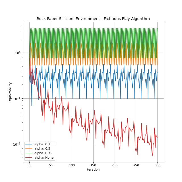
Fictitious Play

For detailed explanation of the algorithm, you can refer to Perrin et al.[1]. The implementation of Fictitious Play in this library is based on Fictitious Play Damped introduced in Perolat et al.[2]. The damped version generalizes the original algorithm by adding a learning rate parameter \(\alpha\). It is worth mentioning that the Fixed Point Iteration algorithm is a special case of Fictitious Play Damped with \(\alpha=1\).

Hyperparameters:

• alpha: The learning rate. It can be any number in \([0, 1]\) or None. If None, the implementation would be inline with the original Fictitious Play algorithm as the learning rate used in the \(n^{\mathrm{th}}\) iteration would be \(\frac{1}{n+1}\). The default is None.

You can create an instance by importing and instantiating FictitiousPlay. Let’s see this algorithm in action.

(png, hires.png, pdf)

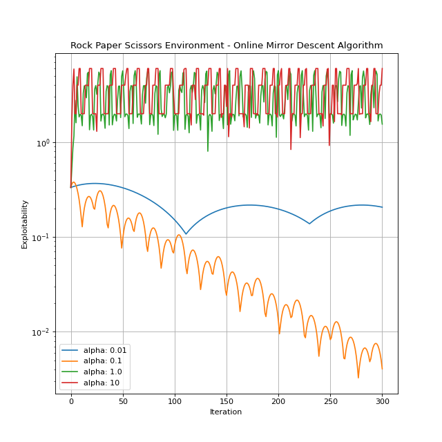
Online Mirror Descent

You can refer to Perolat et al.[2] for a detailed explanation.

Hyperparameters:

• alpha: The learning rate. The default is 1.0.

Let’s see how Online Mirror Descent performs.

(png, hires.png, pdf)

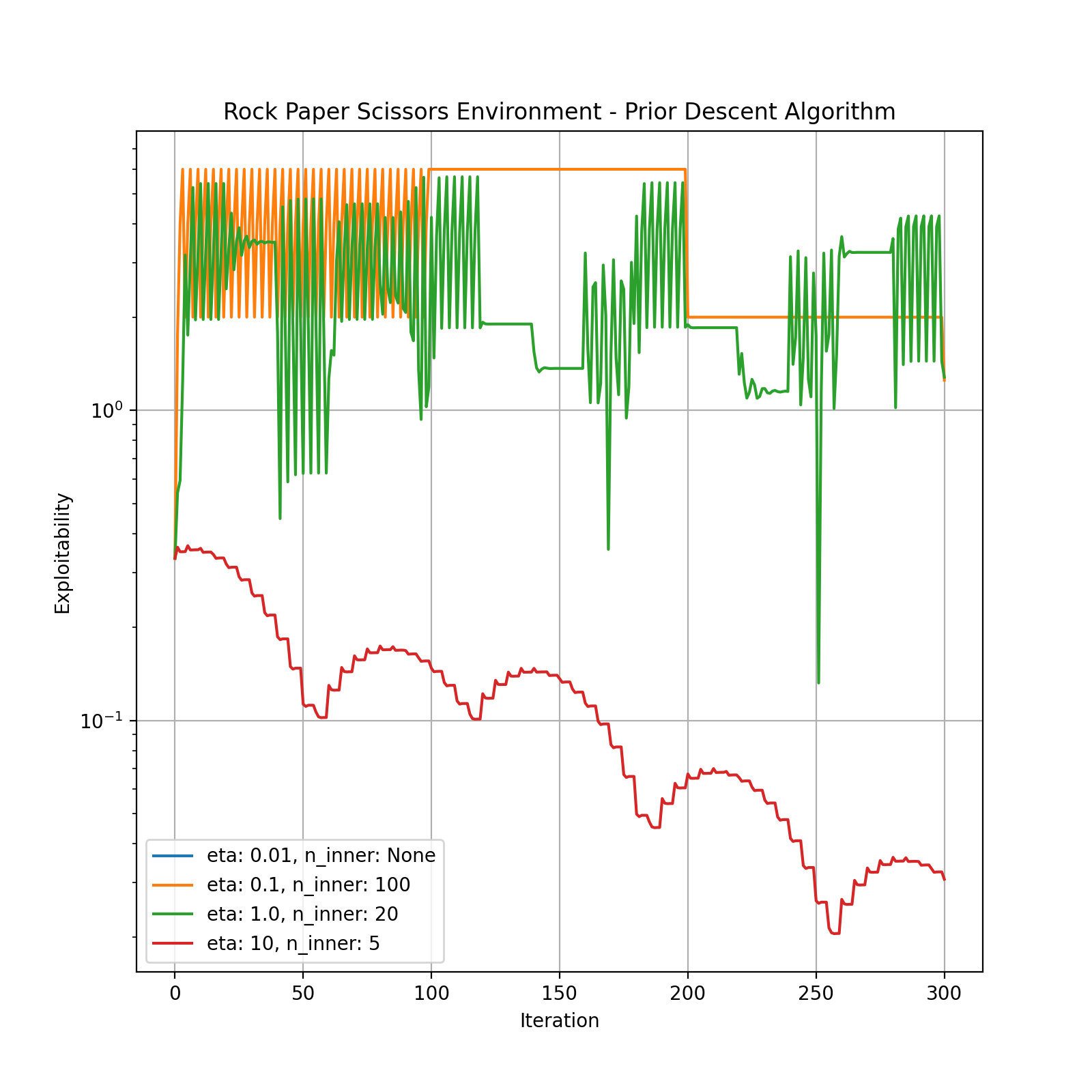
Prior Descent

The algorithm is explained in detail by Cui and Koeppl[3].

Hyperparameters:

• eta: The temperature. It can be any positive number. The default is 1.0.

• n_inner: Determines the number of iterations between prior updates. It can be a positive integer or None. If None, prior remains intact, which is basically the GMF-V algorithm Guo et al.[5].

You can create an instance by importing and instantiating PriorDescent. Let’s give it a run.

(png, hires.png, pdf)

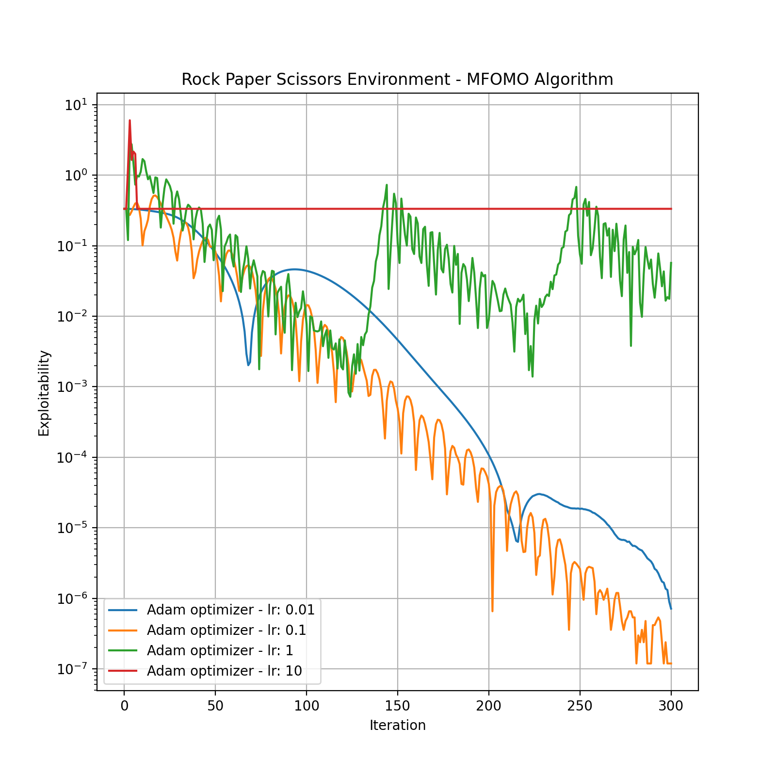
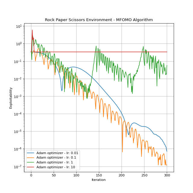
Mean-Field Occupation Measure Optimization (MFOMO)

The algorithm is introduced and explained in details in Guo et al.[4].

Hyperparameters:

MFOMO has several hyperparameters, each of which plays an important role in the algorithm performance. Below, only one of them is described. Detailed information on the rest of the hyperparameters is provided in the More on MFOMO subsection.

• optimizer: Determines the optimization algorithm and its configuration. optimizer should be a dictionary with two keys:

  1. "name": The name of a PyTorch optimizer, e.g., Adam, SGD, RMSprop, etc.

  2. "config": The desired configuration for the selected optimizer. For example, if we choose Adam, then we can set the value of "config" as {"lr": 0.1, "amsgrad": True}.

  By default, it is set to {"name": "Adam", "config": {"lr": 0.1}}.

You can create an instance by importing and instantiating MFOMO. Let’s see this algorithm in action.

(png, hires.png, pdf)

Tuning

As you may have noticed in the previous section, choosing the right set hyperparameters is essential to get the best performance out of an algorithm. A set of hyperparameters could work for one environment but result in a poor performance in other environments. Even two distinct instances of the same environment could require very different sets of hyperparameters. Accordingly, manually tuning the hyperparameters for algorithms such as Fictitious Play and Online Mirror Descent, despite having only one tunable parameter, is not very straight forward, let alone for Prior Descent and specifically for MFOMO that have several hyperparameters with a wide value range.

All the algorithms in MFGLib are endowed with a built-in tuner which could be used to tune the algorithms on one single environment instance or a suite of several environment instances. The tuners are based on Optuna (Akiba et al.[6]), an open source hyperparameter optimization framework used to automate hyperparameter search. You just need to call the tune() method to start the tuning process. Let’s take a closer look at the tune() method and its input arguments.

• env_suite: This is the list of environments we want to tune our algorithm on.

• max_iter: This determines for how many iterations each algorithm trial should be run on each environment instance in the environment suite.

• atol and rtol: Determine the early stopping parameters.

Solved/Unsolved Environment Instances: While running an algorithm on an environment instance, if the exploitability level reaches or goes below atol + rtol * score_0, where score_0 is the initial exploitability, we consider the environment instance solved by the algorithm. Otherwise, we mark it as unsolved.

Stopping Iteration: When an algorithm is run on an environment instance, stopping iteration is the number of iterations needed for the algorithm to reach the desired exploitability level (atol + rtol * score_0). If the algorithm does not reach this level in less than max_iter iterations, we set the stopping iteration to max_iter.

• metric: Determines the metric used by the tuner–the tuner searches for a set of hyperparameters that minimizes the given metric. The two supported options are listed below:

  1. "shifted_geo_mean": Assume that we have \(n\) environment instances in the environment suite and an algorithm is run on all these instances. Let’s denote by \(s_1, s_2, ..., s_n\) the stopping iterations corresponding to these environment instances. Then, a way to evaluate the performance of the algorithm on the whole environment suite is to consider the shifted geometric mean of the stopping iterations. To be precise, we consider \(\sqrt[n]{(s_1+m)(s_2+m)...(s_n+m)}-m\), where \(m\) is the shift parameter. Note that \(s_i\) are non-negative numbers less than or equal to max_iter. Therefore, the shifted geometric mean would be a non-negative number less than or equal to max_iter.

  2. "failure_rate": This metric determines the portion of instances in the environment suite NOT solved by the algorithm, which will be a number in \([0, 1]\).

• n_trials: The number of trials. If this argument is not given, as many trials are run as possible.

• timeout: Stop tuning after the given number of second(s).

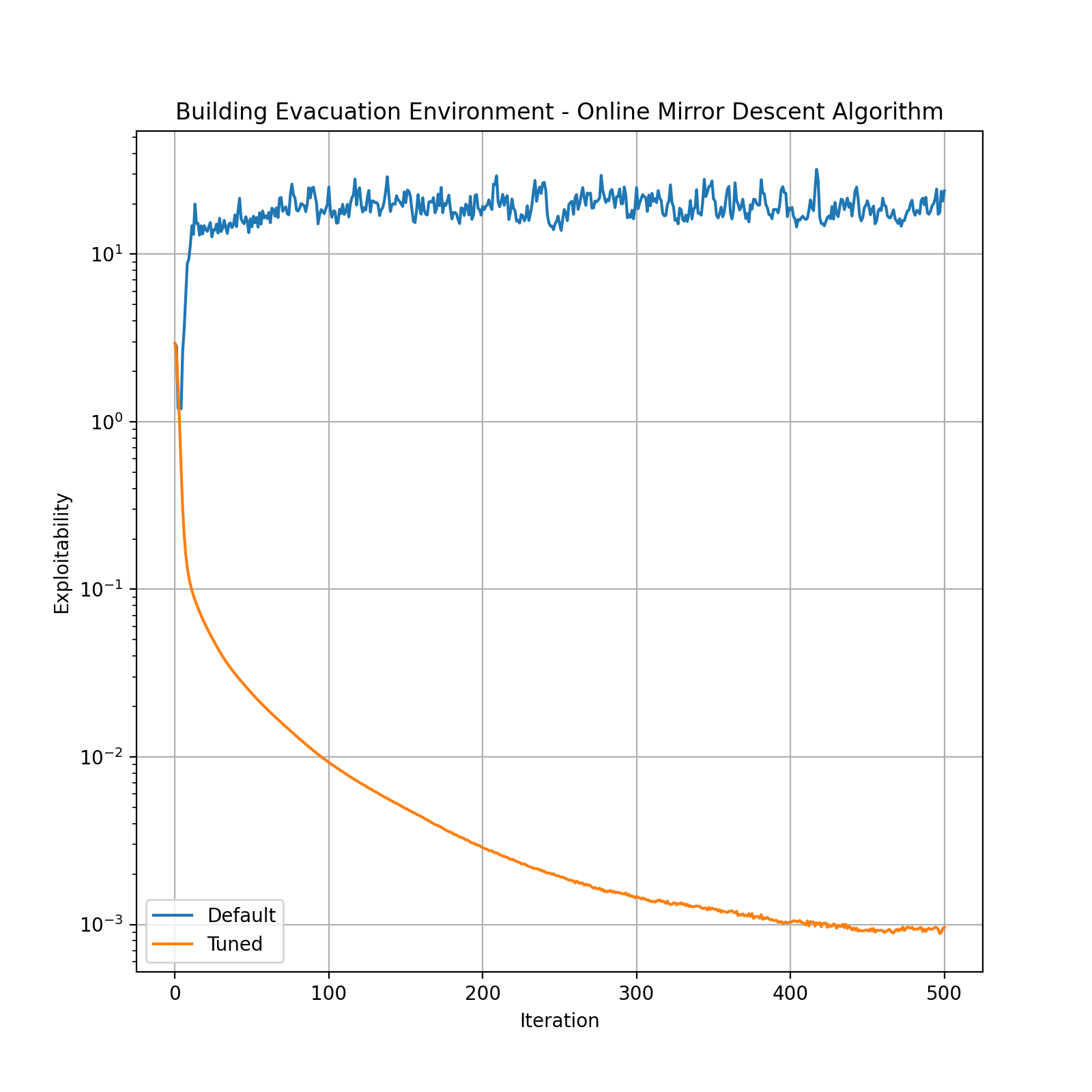
To demonstrate how the tuner works, let’s consider an instance of the Building Evacuation environment and tune the Online Mirror Descent algorithm on it. We will compare the performance of the tuned and default algorithms.

The tuner runs for 20 trials and the time limit is 60 seconds. Note that env_suite=[Environment.building_evacuation(T=5, n_floor=10, floor_l=5, floor_w=5)] as we want to tune the algorithm only on one specific environment instance.

from mfglib.env import Environment

from mfglib.alg import OnlineMirrorDescent

# Default algorithm
online_mirror_descent = OnlineMirrorDescent()

# Tuned algorithm
online_mirror_descent_tuned = online_mirror_descent.tune(
             env_suite=[
                 Environment.building_evacuation(T=5, n_floor=10, floor_l=5, floor_w=5)
             ],
             max_iter=500,
             atol=0,
             rtol=1e-2,
             metric="shifted_geo_mean",
             n_trials=20,
             timeout=60,
     )

(png, hires.png, pdf)

The tuned algorithm outperforms the default. By setting lower exploitability thresholds, we might get even a better performance, but we may need to run the tuner for more trials and time.

A few remarks about the tuner:

1. To ensure that the tuned hyperparameters work well on a broader range of environments, we can pass a list of multiple environment instances to the tuner via the env_suite input argument.

2. The default set of hyperparameters may not be used during the tuning process. Consequently, there might be cases in which the default algorithm outperforms the tuned algorithm.

3. Depending on the the values of the tuner’s inputs such as max_iter, atol, rtol, etc., it is possible that none of the algorithm trials solve any of the environment instances in which case the tuner does nothing. However, if at least one of the algorithm trials is successful in solving at least one of the instances, then tuner outputs the algorithm equipped with the best set of hyperparameters.

4. An algorithms’ tuner conducts hyperparameter search for all the existing hyperparameters and over predetermined search domains, which is determined via the _tuner_instance() method. By modifying this method and adapt the tune() method to these changes, one can change the set of tunable hyperparameters as well as their corresponding search domains.

More on MFOMO

MFOMO reformulates the problem of finding the NE solutions of an MFG as an optimization problem. To be precise, finding an NE solution of an MFG is equivalent to solving the following constrained optimization problem:

(1)\[\begin{split}\text{minimize}_{L, z, y} \quad &||A_LL-b||_2^2 + ||A_L^Ty + z - c_L||_2^2 + z^TL\\ \text{subject to} \quad &L\geq 0, ~ 1^TL_t=1 ~ \forall t \in \{0, ..., T\},\\ &1^Tz \leq SA(T^2+T+2)r_{\max},\\ &||y||_2\leq \frac{S(T+1)(T+2)}{2}r_{\max}.\end{split}\]

For detailed description of the variables and parameters in this optimization formulation, please refer to Guo et al.[4].

We can solve (1) using an optimization algorithm such as Projected Gradient Descent. Furthermore, Guo et al.[4] suggests several techniques using which could result in an improvment in the convergence. By modifying the corresponding input parameters, you can change the optimizer and/or enable different techniques to be used while running MFOMO. In what follows, we categorize the algorithm hyperparameters based on their usage and describe them.

Optimization Algorithm: You can run MFOMO with different optimization algorithms. Currently, we only support PyTorch optimizers. The following input argument allows you to set your desired optimizer:

• optimizer: Determines the optimization algorithm and its configuration. optimizer should be a dictionary with two keys:

1. "name": The name of a PyTorch optimizer, e.g., Adam, SGD, RMSprop, etc.

2. "config": The desired configuration for the selected optimizer. For example, if we choose Adam, then we can set the value of "config" as {"lr": 0.1, "amsgrad":True}.

By default, optimizer is set to {"name": "Adam", "config": {"lr": 0.1}}.

Note

Since we are solving a constrained optimization problem, the optimizer iterations are automatically projected onto the constraint set after each iteration.

Parameterized Formulation: Replacing the constrained optimization problem (1) with a smooth unconstrained problem enables us to use a broader range of optimization solvers. As explained in Appendix A.3 of Guo et al.[4], we can reparameterize the variables in MFOMO to completely get rid of the constraints. The new problem is called the “parameterized” formulation. Using the following input argument, we can switch between the different formulations:

• parameterize: Optionally solve the alternate “parameterized” formulation. Default is False.

Hat Initialization:

• hat_init: Determines whether to use “hat initialization”, in which, given the initial mean-field \(L\), initial \(z, y\) are set to \(\hat{z}(L), \hat{y}(L)\) as explained in Proposition 6 of Guo et al.[4]. Default is False.

Redesigned Objective: In the optimization problem (1), one can assign different coefficients to the three terms in the objective function, and come up with a “redesigned objective”. To be precise, the redesigned objective is \(c_1 ||A_LL-b||_2^2 + c_2 ||A_L^Ty + z - c_L||_2^2 + c_3 z^TL.\)

We can also apply different norms (L1 or L2) to the objective terms. The following input arguments determine the parameters of the redesigned objective:

• c1, c2, c3: The redesigned objective coefficients. Default is 1 for all the coefficients.

Note

Without loss of generality, we can always let c3=1.

• loss: Determines the type of norm (L1, L2, or both) used in the redesigned objective function. Three available options are listed below:

1. "l1": The objective will be \(c_1 ||A_LL-b||_1 + c_2 ||A_L^Ty + z - c_L||_1 + c_3 z^TL\).

2. "l2": The objective will be \(c_1 ||A_LL-b||_2^2 + c_2 ||A_L^Ty + z - c_L||_2^2 + c_3 (z^TL)^2\).

3. "l1_l2": The objective will be \(c_1 ||A_LL-b||_2^2 + c_2 ||A_L^Ty + z - c_L||_2^2 + c_3 z^TL\).

The default is "l1_l2".

Adaptive Residual Balancing: We can adaptively change the coefficients (\(c1\), \(c2\), and \(c3\)) of the redesigned objective based on the value of their corresponding objective term. This can be done using the following input arguments:

• m1, m2, m3: Determine the parameters used for adaptive residual balancing.

Let’s denote by \(O_1\) the value of the first objective term (depending on the norm used, it could be either \(||A_LL-b||_1\) or \(||A_LL-b||_2^2\)), and let \(O_2\) and \(O_3\) be the values of the second and third objective terms, respecively. When adaptive residual balancing is applied, we modify the coefficients in the followin cases:

1. If \(O_1/ \max(O_2, O_3) > m_1\), then multiply c1 by m2.

2. If \(O_1/ \min(O_2, O_3) < m_3\), then divide c1 by m2.

3. If \(O_2/ \max(O_1, O_3) > m_1\), then multiply c2 by m2.

4. If \(O_2/ \max(O_1, O_3) > m_3\), then divide c2 by m2.

• rb_freq: Determines the frequency of residual balancing. It can be a positive integer or None. If None, residual balancing will not be applied.

Initialization: We can set the initial policy for any algorithm using the input argument pi through the solve() method. MFOMO uses the initial policy to compute the initial values of the variables \(L\), \(z\), and \(y\). However, if you want to initialize these variables directly, you can do so using the following input arguments:

• L, z, y: The initial values of math:L, \(z\), and \(y\). Default is None. If not None, these values overwrite the initial values derived from the initial policy.

• u, v, w: The initial values of the variables math:u, \(v\), and \(w\) used in the “parameterized” formulation. Refer to the Appendix A.3 of Guo et al.[4] for more information. Default is None. If not None, these values overwrite the initial values derived from the initial policy.

References

[1] (1,2)

Sarah Perrin, Julien Perolat, Mathieu Laurière, Matthieu Geist, Romuald Elie, and Olivier Pietquin. Fictitious play for mean field games: Continuous time analysis and applications. 2020. arXiv:2007.03458.

[2] (1,2,3)

Julien Perolat, Sarah Perrin, Romuald Elie, Mathieu Laurière, Georgios Piliouras, Matthieu Geist, Karl Tuyls, and Olivier Pietquin. Scaling up mean field games with online mirror descent. 2021. URL: https://arxiv.org/abs/2103.00623, doi:10.48550/ARXIV.2103.00623.

[3] (1,2)

Kai Cui and Heinz Koeppl. Approximately solving mean field games via entropy-regularized deep reinforcement learning. In Arindam Banerjee and Kenji Fukumizu, editors, Proceedings of The 24th International Conference on Artificial Intelligence and Statistics, volume 130 of Proceedings of Machine Learning Research, 1909–1917. PMLR, 13–15 Apr 2021. URL: https://proceedings.mlr.press/v130/cui21a.html.

[4] (1,2,3,4,5,6,7)

Xin Guo, Anran Hu, and Junzi Zhang. MF-OMO: an optimization formulation of mean-field games. 2022. URL: https://arxiv.org/abs/2206.09608, doi:10.48550/ARXIV.2206.09608.

[5]

Xin Guo, Anran Hu, Renyuan Xu, and Junzi Zhang. Learning mean-field games. 2021. arXiv:1901.09585.

[6]

Takuya Akiba, Shotaro Sano, Toshihiko Yanase, Takeru Ohta, and Masanori Koyama. Optuna: A next-generation hyperparameter optimization framework. In Proceedings of the 25th ACM SIGKDD International Conference on Knowledge Discovery and Data Mining. 2019.